Up to this point I had only looked at stateless neural networks, such as feed-forward nets. This means that the network treats every input vector independent of every other. This is quite limiting when dealing with certain tasks where the input is not naturally a fixed-length vector, but is a stream of correlated data (eg: sentiment analysis based on the words of a document). Recurrent Neural Networks are a class of network that process data as a stream, one element at a time, keeping some internal state or memory between time steps. This class of neural network is very interesting as it can learn a hidden state representation necessary for a particular task. To me the most interesting application of RNNs would be for Reinforcement Learning an agent policy in a Partially Observable Markov Decision Process (POMDP), removing the need to explicitly model and track the hidden state. I’ll explore applying RNNs to this type of problem for a later project, for now I’m going to look into the basics of training an RNN.

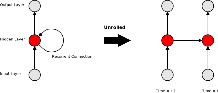
In terms of implementation RNNs are quite similar to feed-forward nets, the main difference being that the connections between nodes can span across time-steps. In a feed-forward network the inputs for a particular node are the weighted outputs of nodes from the previous layer. In a recurrent neural network the inputs for a node can also include the weighted outputs of nodes from a previous time-step. Implementation wise the forward pass for an RNN is almost the same as a FNN, the only addition is that when a stream of input vectors is processed, the activation state of the nodes is stored, to be used when processing the next input vector. This “unrolling” of the recurrent connection is illustrated in the diagram below.

Training an RNN

Training an RNN can be done with gradient descent, using a variant of Back-Propagation, called Back-Propagation Through Time (BPTT), to calculate the gradient for a given input/output sample. In this case we calculate the gradient not for a single training input/output vector pair, but for an ordered series of vector pairs sampled from a stream (I’ll refer to this series of input/output pairs as a chunk). This is how an RNN learns dependencies between elements of a series. The length of the ordered series is limited to some maximum length for reasons of computational complexity (training time scales linearly with the chunk length) and memory complexity (which also scales linearly with chunk length). It is important to note that the RNN can only learn a dependency going back in time no longer than the length of the series used for BPTT.

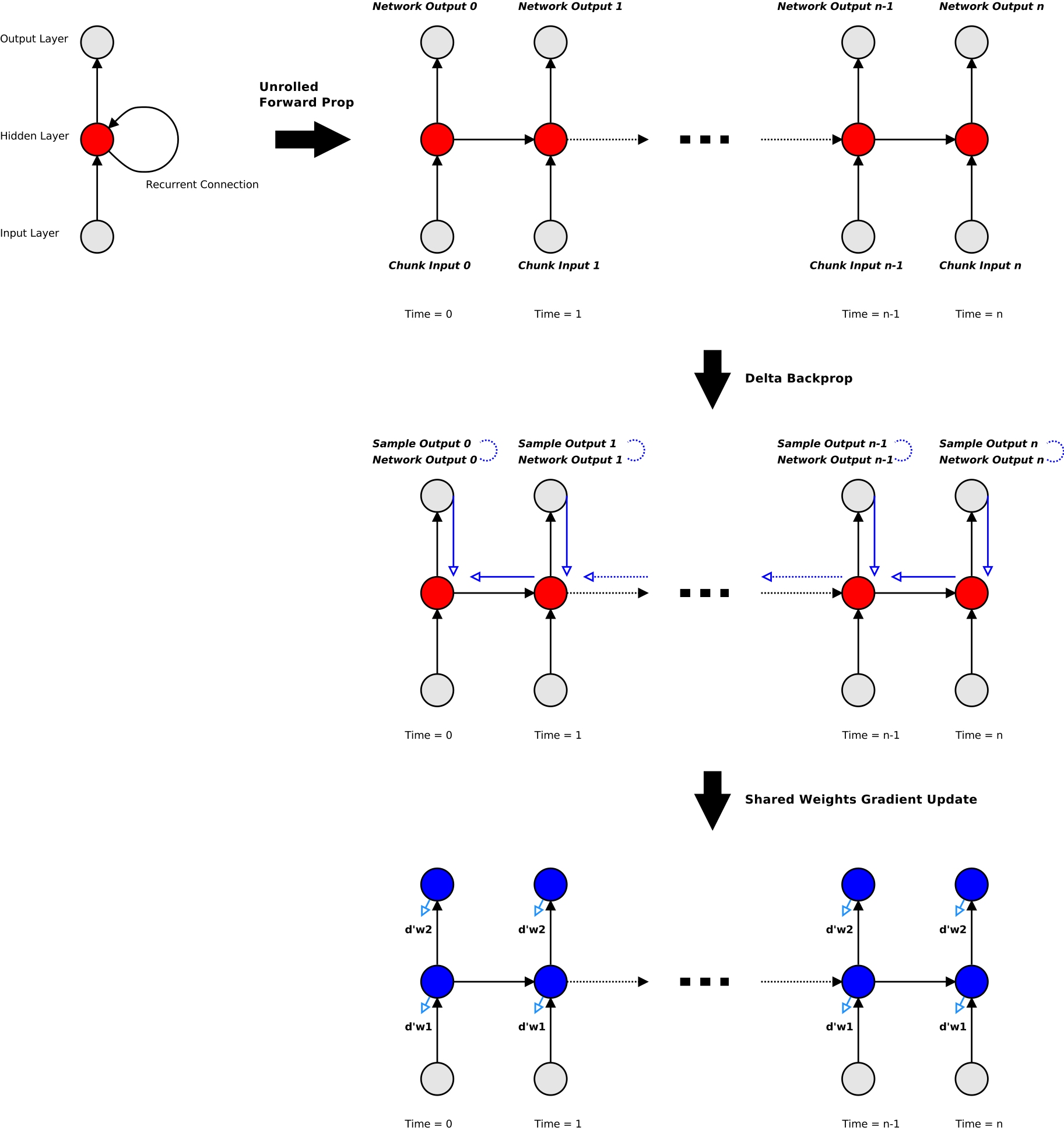
Implementing BPTT is a three step process:

• The first is unrolling the network forward propagation step over the training chunk.
• The second is back-propagating the errors through the unrolled network, aggregating the layer deltas for each layer/timestep pair.
• The third is calculating the gradient matrix for each layer connection by taking the average contribution of the layer deltas across the entire chunk.

This process is represented in the below diagram. Implementing BPTT is not very complicated, requiring only a little extra book-keeping and lookups as compared to vanilla back-propagation. The final result of BPTT is a tensor of weight gradients over the given training chunk. Just like with feed-forward nets, this gradient tensor can be used either directly for stochastic gradient descent, or for some stateful algorithm like ADAM or Adagrad.

When training an RNN, as with other neural networks, regularisation can help improve the performance of the resultant network. L1 and L2 regularisation work as usual, but for drop-out regularisation it is recommended to only apply drop-out for non-recurrent connections. This relatively simple concept actually complicated my implementation a fair bit. I could no longer store a single output vector per layer, but had to model the inter-layer connections explicitly, with each storing the weighted activations of the source layer. I would then apply drop-out to the non-recurrent connections. This meant that the memory requirements for this data scaled linearly with the number of connections, rather than the number of layers (as well as requiring some extra memory copying).

Sample Task

The specific task I used to test my RNN implementation is character level language modelling. This involves taking a large text corpus (eg: all of the works of Shakespeare, or a dump of Wikipedia), encoding every character as a 1-hot vector, and learning to predict the next character in the text stream. The input series is 1-hot encoded vector of the current character, and the output series is the 1-hot encoded following character. For the BPTT algorithm I used a chunk length of 16 characters (so at most my network could learn character dependency across 16 letters). I played around with a few different network configurations, usually about 2 hidden layers of about 128 or 256 nodes each, with a recurrent self-connections for each. The output layer is a softmax layer. I tried a few different activation functions, Logistic, Tanh, ReLU and ELU. I didn’t have a concrete evaluation measure in place, simply sampling from the resultant network to get a piece of ‘creative writing’, and therefore I couldn’t see an obvious winner between the different activation functions. Below is an example sampled text from an RNN trained on the works of Shakespeare:

i do now stood i’ tear and kneel my earth and tall so; you meather i would come whom the world you sir. exeunt. others phaketh should those harryworn and but lartius. rom. i am drunk’st if you do and will coriolanus. where heaven deserve or loving of his percy done at this scene in himself bears to kiss is true apollaysarty and in a pluckedner’s grosser for him. fair gentleman. and ancient slodky deny so forswey heaven: elsewis. enter alms by some enter pipe ere liberty and that is the rushes and loving it my rich put warwick thou stratch’d my need himself mine. for foisers a brain hands? i love thy faith. shylock? princes cannot spoke of mincius and are as messand good and be fight will not do tains. prince a rich blastian. sir rough be death on and she met the were a pale this you and drawn’s stewarwand i am mine enter shall therefore my lord ‘em. what of my dread my heart!

As can be seen, the text definitely has a “Shakespearean” quality to it, despite being largely nonsense with no real structure. Still, not bad for purely character-level language modelling with a simple RNN.

Thoughts and Future Work

There are a few practical problems with RNNs. First is that they take a long time to train. At a high level, if we use training chunks of say length 16, then each iteration of BPTT over the network will take more than 16x as long as a back-propagation iteration over a feed-forward network of the same layout (but without the recurrent connections). Here I’m just talking about the computation of a single gradient, not comparing the quality of the resultant networks or the number of iterations required for each to converge. But to make it even worse, RNNs typically require more iterations of gradient descent to converge to a good set of weights, making them computationally even more expensive. One of the reasons for this is the vanishing gradient problem (I should also mention exploding gradients as another potential source of trouble, but relatively easily handled with gradient clipping). With long-term dependencies we must propagate the error through the network for many time-steps (the length of the chunk). At each step the delta magnitude is potentially reduced due to the derivative of the activation function being <= 1. This means that by the time the delta is propagated from the most recent chunk time-slice to the oldest slice, its magnitude may be very small or even 0 (due to rounding). This vanishing gradient problem with long-term dependencies is addressed by several variants of RNNS such as Long Short Term Memory (LSTM) and Gated Recurrent Unit (GRU) networks. These feature an arrangement of nodes and connections to implement what is essentially a differentiable latch or flip-flop. This allows the network to far more easily “remember” information, and thus better handle long-term dependencies. I will explore these networks in detail in the future.

The code for this project can be found on Github: here (warning: code is experimental and may be slightly messy).