Having done some work with Recurrent Neural Networks and implemented several variations, it was time to apply them to something more interesting than character-level language modeling. To me one of the most interesting applications of RNNs is for agent control in a Partially Observable Markov Decision Process (POMDP). First, what is a POMDP? A Markov Decision Process (MDP) is a stochastic control process, where you are in some state s and you can perform some action a. This action will result in a transition into a new state s’ and a reward r. Both of these are dependent only on the tuple (s, a), rather than on the history of states and actions (this is known as the Markov Property). A POMDP is a generalisation of MDPs in that it introduces the concept of observations and the possibility that the current state s can only be deduced from observations, rather than being directly observable. In this case the agent must maintain some internal probability distribution over the states s, and integrate the observations at every time step to update this distribution. The ultimate task of an agent in a MDP and POMDP is to choose actions such that the long term reward is maximised.

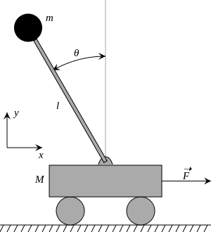
A simple example of an MDP is balancing an inverted pendulum. In this type of system the state can be expressed as the weights and dimensions of the cart/pendulum system, the current angle of the pendulum, and its current angular velocity. This state information can be used to decide on an action, in the form of motor-drive applied to the cart’s wheels, that will keep the pendulum upright. This simple MDP problem can be converted into a POMDP by removing the current angular velocity of the pendulum from the observed state. In this case we would need to integrate the observations of the pendulum angle over time to keep track of a state representation necessary for making an optimal action decision.

For this project I chose to implement a Reinforcement Learner agent for controlling an inverted pendulum cart. I would use a Recurrent Neural Network to learn a Q-function, mapping observations to action values. I used aspects of DQN learning to train the RNN.

The most interesting aspect of this task is that usually when dealing with a POMDP you have to make explicit decision as to how to integrate the observations over time, how to deal with the state uncertainty, and how to internally represent the state to attain the Markov Property for the decision process. Using an RNN for this task removes much of these decisions. In theory the RNN can learn to do all of this implicitly.

Simulation Setup

The first thing to do is to set up a way of simulating the behaviour of a cart and inverted pendulum system. I decided to use the Bullet Physics library as I was already familiar with it, having used it for one of my PhD projects. The Bullet library allows easy simulation of rigid body dynamics, modelling various shapes and linkages/constraints. The cart is modelled as a box with 4 wheels, and the pendulum is modelled as a weighted long and thin cylinder attached with a hinge joint to the top of the cart. The simulation world contains a pendulum cart on a z-plane, with 2 immovable boxes some distance either side of the cart. These boxes are there to restrict the maximum displacement of the cart, which should make the control task potentially slightly harder. This cart system is modelled at a sampling rate of 30 times a second using the default discrete solver for Bullet.

In addition to modelling the dynamics of the cart/pendulum system I also added a “wind” components. During each simulation step I apply a random (parametrisable) impulse to the top of the pendulum. The idea here is to add some unpredictability to the system, complicating the balancing task for the controller.

Agent Interface

In a system control task we must define an interface for the agent to observe some aspects of the current state, and an interface for the agent to affect the system. For the balancing task I defined the agent observations and actions as follows:

• Observations: (x,y) positions of the cart and pendulum top.
• Actions: apply one of the following impulses to the cart [0, 10, -10, 20, -20, 40, -40].
• Rewards: 0 if the angle of the pendulum is within 60 degrees of vertical, otherwise -1.

With the agent observations it is important to note two things: the angle of the pendulum is not directly observed (only the cart base and pendulum top x,y coordinates), and velocities are not observed (only instantaneous positions). This implies two things: the agent would need to relate the cart and pendulum positions to derive the pendulum angle, and the agent would need to integrate observations from different times to derive any linear or angular velocity measures.

The interface between the agent and the simulation is such that the agent can observe the world at a rate of once per second, and apply an action once per second. This rate is deliberately lower than the simulation rate, further complicating the agent’s task as it cannot make very many fine adjustments but rather has to plan ahead, making use of fewer adjustments.

Policy Training

The agent’s policy is controlled by a Q-function modelled by a Recurrent Neural Network. This network has 4 inputs, being the raw observations described above, and the output is the vector of Q-values of the 7 available actions. I ended up using a network with 2 hidden layers, each with 64 nodes and a tanh activation function. The second of the two hidden layers has a recurrent self-connection.

Training of this RNN is done in a similar way to my previous DQN project (in that case I was training a Feed-Forward Neural Network to play Connect Four). The training is done by having a separate “Experience Memory” that is used to provide randomly sampled experience “traces” (series of state observations and rewards) for batch training. The Experience Memory is continuously being added to by a playout thread, which is generating new experiences by running many simulations. The playout controller uses a “reference” version of the RNN. A separate training thread is using the sampled traces from the Experience memory to train a “learning” RNN. This RNN is trying to learn the Q-function of actions given an observation (and the current state of the network). The target Q-function is provided by the “reference” RNN. Every 5000 iterations the “reference” RNN is updated to be equal to the “learning” RNN. The combination of an experience memory and the separation of learning and target networks are the two key tenets of “Deep Q-Learning”, and help reduce any feedback instabilities that would otherwise arise.

The network was trained for 200,000 iterations, with the end result being a fairly good pendulum balancing policy. You can view a video of the learned RNN in action:

To reach this end result took a decent amount of work. For a long time I could not get the network to learn a good Q-function, and the agent could not balance the pendulum. I thought it may be some instabilities due to the Recurrent network, but it seemed like the gradient magnitudes were reasonable. I tried many different parameters for Experience Memory size, rate of update of the “reference” network, etc. At some point I gave up on Q-learning, and tried SARSA (as well as some hacky variants of TD learning) in the hope that it would be more stable and produce an acceptable policy. However, in the end I was able to figure out a couple of fundamental mistakes I was making in my initial attempts, eventually getting the Q-learning to work.

Lessons Learned

While working on this project I ran into several problems and learned a few lessons the hard way (after banging my head against the problem for a while). Most are obvious in hindsight, but thats usually how it works:

1. decaying the learn rate is important in the context of RL. This is a lesson I forgot, and initially just defaulted to using ADAM gradient descent. However, since an RL agent is learning (gradually doing more exploitation than exploration), the distribution of examples shown to the NN is changing. This means that unless the learn rate decays, the neural network will tend to “forget” what it learned in the past.
   • more recurrent connections in a RNN can lead to worse performance.
   • “normalised” rewards can improve learning. I found that using rewards of [0.5, -0.5] for an upright/fallen pole worked better than rewards of [0, -1].
   • the “trace” length used for the BPTT algorithm must be long enough to capture (action -> reward) causation. Initially I was using a rather short “trace” length of 8. In this case the eventual behaviour was that the agent tended to make a very poor first action (say a large push), and then spend the subsequent time trying to save itself. This turned out to be because it was taking more than 8 observations for the pole to fall (and thus earn a penalty), so the agent was never able to learn the causation between a large initial cart push, and the pole eventually falling down. Increasing the “trace” length solved this problem.

Future Work

All in all, this has been one of the most fun and interesting projects I’ve done so far. I can see a number of areas for future projects in this direction. The first is to use a more sophisticated RNN structure, such as LSTM or GRU. This should allow for more effective learning of long term dependencies between actions and rewards. The second is to approach a more difficult control/decision problem. Inverted pendulum control is a useful demonstration problem, but a more complex virtual world (potentially with opponents) would be massively interesting to play around with.

The code for this project can be found on Github: here (warning: code is experimental and may be slightly messy).