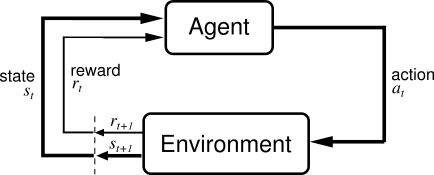
Reinforcement learning is an interesting learning paradigm, distinct from supervised and unsupervised learning. Supervised learning features an external source providing the learner with the correct/desired classification/value/action for a given input, and the learner’s aim is to learn this mapping and be able to apply it at a later time. Unsupervised learning is concerned with extracting structure and information from input, without having access to a ground truth. Clustering and dimensionality reduction are two examples. Reinforcement learning deals with an agent in some environment, performing actions and obtaining rewards. The agent’s goal is to carry out an action policy that maximises long term reward. The main distinction from say supervised learning is that there is no data given to the agent as to what action to perform for various environment states. Instead the agent has to explore different actions to discover their effects, experimenting to discern good and bad actions. Another distinct issue is reward assignment. An agent may only rarely receive rewards from the environment, relative to the frequency of actions performed. This means that it may not be directly clear which actions lead to the reward. A simple example is a chess playing agent. The environment is the chess board, and the actions are individual moves. Rewards are assignment for winning or losing a game (losing would result in negative reward), but not for intermediate board states.

Background

I’ll start off by referring to a very good online course on Reinforcement Learning by David Silver. It covers this topic very well.

RL is a method of solving a Markov Decision Process (MDP). An MDP is a stochastic control process where at each time step the agent is in some state s and may choose some action a. This will probabilistically transition the agent into the next state s’ and give some reward as a function of the transition R(s, a). The crucial property is that the transition obeys the Markov property. This means that the transition and reward probabilities are only dependent on the pair (s,a), and are not dependent on the entire history of previous states. Basically, the state s should encode all of the important information to be able to make a good decision on which action to take.

Broadly speaking, RL methods can be broken up into two groups, policy and value function methods. Policy methods perform a search in policy space, whereas value function methods try to estimate the value function. The value function is a function that tries to estimate the long-term utility of either a state, or a state-action pair, and the agent simply selects the arg-max action over this function. This is the approach that I will pay most attention to here.

Broadly speaking (in very very general terms) a lot of value function algorithms in RL work as follows:

• the agent stochastically follows the current policy as defined by the current value function
• whenever a reward is received the agent propagates it back through its history, assigning each action some of the reward
• over time, this gives the agent a good idea of what states and actions result in good rewards.

Exploration vs Exploitation

One of the dilemmas of any RL task is that of exploration vs exploration. Since there is no externally provided data available to the agent as to which action to choose for a given state (or the value of the state-action pair), the agent must perform some exploration. It should try out different actions in different states to explore the space and find out which actions pay off and which don’t. However, by doing pure exploration the agent is foregoing rewards that it would have received had it followed the optimal policy according to its current knowledge. Therefore the agent must balance these two competing desires. Two fairly simple, yet effective, approaches to this are e-greedy and softmax action selection.

E-Greedy

The e-greedy algorithm is extremely simple. Simply put, for every action decision the agent has some probability e of taking a completely random action, and a 1-e probability of taking the action with the highest value. Sometimes e is a fixed value, and sometimes it starts off high and undergoes a gradual decay over agent training epochs.

Softmax Weighting

Another common approach is to assign a weight to each action depending on its value. A random action is chosen, with the probability of choosing any one action proportional to its weight. These weights are usually not directly proportional to the action values, but are rather passed through a softmax function with a temperature. The temperature variable controls how biased the resulting distribution is toward the higher value actions. Typically this temperature variable starts off high and decays during the training epochs.

Q-Learning

Q-learning is a popular model-free reinforcement learning technique (model free here means that the Markov process of state transitions is not explicitly modelled). The aim of q-learning is to learn the function Q(s, a) that returns the expected value of the immediate reward from performing action a in state s, plus the discounted rewards received by following the optimal policy thereafter. The algorithm is roughly as follows:

1. initialise some starting version of the Q-function
2. perform actions in the environment according to some exploration/exploitation policy (e-greedy, softmax, etc)
3. take every transition (s, a, s’, r), where s is the state, a is the action taken, s’ is the resulting state, and r is the immediate reward. Shift the q-value Q(s, a) toward r + g * argmax[a] Q(s’, a’), where g is the discount factor over future rewards.
4. gradually decrease the exploration factor (whether epsilon in e-greedy or the temperature in softmax).

This fairly simple learning algorithm can do a good job of learning an effective policy for an MDP task. One of the key features of Q-learning is that is features off-policy learning. This comes about from the use of argmax over all actions in the state s’ in the Q update function. The argmax action may be different to the actual action performed during that episode of learning, hence “off-policy”.

Grid World

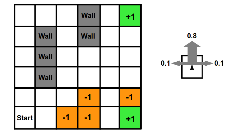
To play around with these concepts, the simplest application of RL I could think of is a grid world environment. A grid world is basically a 2D maze for an agent to navigate, with some “exit” cell offering a positive reward, and optionally some cells offering a penalty. The agent’s task is to learn to navigate this world to find the “exit”, while avoiding the penalty cells. This is a very common example task for RL, used in many lectures/courses. I think the best thing about this toy problem is it is simple enough to effectively visualise and see whether an RL implementation is working as intended. To that end, this was the first thing I implemented when starting to play around with RL. The set up is as follows:

1. the agent starts in some cell, each cell is uniquely identifiable
2. each cell allows up to 4 actions (move left, right, up down)
3. when reaching an exit cell, the simulation ends and the agent receives a reward
4. some states give negative rewards
5. the goal of the agent is to learn a policy the reaches the exit cell as fast as possible.

Tic Tac Toe

A more interesting application of reinforcement learning is game playing with an opponent. So rather than having a static environment to explore in a grid world, this instead involves playing a turn-based game against a dynamic opponent. There are countless suitable games, but I chose tic-tac-toe (naughts and crosses) as a first attempt due to its simplicity and small problem space. Another nice property is it’s trivial to see if an agent has converged on the optimal policy, simply by experimentation.

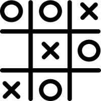
To learn a game policy using RL, there are two options. One is to play against a fixed opponent, say a minimax AI or an agent that simply makes random moves, for example. Another option is for the agent to play against itself. In the latter case we see a big difference between a grid-world scenario and the game scenario in that during learning the “environment” from the agent’s point of view may not be static. As the agent is playing itself and learning, moves and policies that may have been good initially may cease to be so. There is sort of a potential to be chasing one’s own tail, and never settling down on the optimal policy. An interesting thought.

Luckily in this instance I did not have any of these issues and using a simple e-greedy exploration and self-play arrived at the optimal policy for 3x3 tic-tac-toe. The implementation can be found here.

Limitations

The tic-tac-toe and grid world examples have used a table-based Q-function representation. As the states and actions are discrete and small in number, we can store a q-value for each possible state-action pair. However, this obviously does not scale, in terms of space requirements to store the table as well as the time required to explore all state-action pairs. Even a moderately more complex game like Connect-Four is unfeasible using this representation. The solution is to use a function approximation scheme, where we use some function model (eg: linear model) to represent the Q-function, instead of a mapping table. These usually involve extracting some features of the state and action, using those as input to the function to get the value as output. This has two potential up-sides:

1. allow large state and action spaces to be represented without requiring intractable amounts of memory,
2. potentially generalise across states and actions, making educated approximations of Q values for states and actions that may never have been seen during training.

I will cover this in the next topic on Deep Q Learning.

The code for these projects can be found on Github: (here and here) (warning: code is experimental and may be slightly messy).