Restricted Boltzmann Machines (RBM) are an interesting class of neural network, quite different from common feed-forward networks. They played an important part in the evolution of “deep learning”, so I wanted to learn how they worked and play around with an implementation.

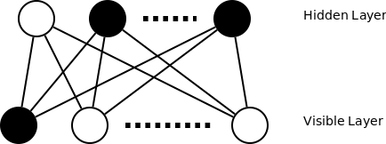
RBMs are a special case of Boltzmann Machines, having come about due to the computational complexity of learning the parameters of a generalised Boltzmann Machine (I won’t go into this aspect any further). An RBM is a generative stochastic neural network, having two layers of fully connected nodes, arranged as a bipartite graph. It is a generative model as opposed to a discriminative one, meaning that its purpose is to model the features and correlations of the input data. This is in contrast to discriminative models which divide the input vector space into regions corresponding to the different target classes. To use a concrete example, a discriminative model may learn that when a certain group of pixels is “on”, then a particular image likely corresponds to the digit “7”; whereas a generative model may learn that when a certain group of pixels is “on”, then another group of pixels is also likely to be “on”. A big plus of generative models is that they can be trained using unlabeled training data, which is typically far easier to obtain compared to labeled examples.

In the original treatment of RBMs, the visible and hidden layer nodes are binary, their value can be either 0 or 1. The network is stochastic in that the value of a hidden node is a random variable with probability of being 1 given by the applying a logistic activation function to the inner product of the incoming weights and the visible layer (plus a bias term):

P(h = 1 | v) = logistic ( bias + weighted sum over v )
P(v = 1 | h) = logistic ( bias + weighted sum over h )

In this way, we can sample the values of the hidden layer, given the a visible vector and the network weights. Symmetrically we can sample the values of the visible layer, if we are given the hidden layer.

So this is all fairly straightforward, but it wasn’t obvious to me what is the point of this type of network. It took some time to form a view of RBMs that made sense to me, but in the end it was all to do with the energy function of the network. The energy function of an RBM is a function of its weights, and the hidden and visible layer vectors.

One way of looking at it is that the energy function tells you how “compatible” the hidden and visible vectors are given a particular RBM. The goal of training an RBM on a particular training set of data is to find network weights that will have a low average energy on the visible vectors (which are sourced from the training data) and the corresponding sampled hidden vectors. The end result of such training should be a network that can output a hidden vector based on a visible vector that has a low resulting energy, if the visible vector has a distribution similar to the training data. Such a hidden vector will correspondingly be an indicator of some correlations (features) present in the visible vector. Basically an RBM is a “feature” detector, where features are correlations between elements of the input vector. For me an intuitive example of this is training an edge (or corner detector), where the visible units are the raw pixels of an image, and the hidden units are detecting the presence of common image features (such as corners and edges), which are essentially correlations between different pixels.

Training

To learn the weights of an RBM we would like to perform gradient descent over the Energy function, similar as with a feed-forward network (except with a FFNN the descent is over the error function). However, it turns out that naively performing gradient descent over the energy function is intractable. This comes about due to the exponential complexity of calculating one of the terms (the normalisation term is the sum over all possible hidden values).

Disclaimer: I’m going to skip over a whole bunch of detail here and massively simplify things, but for a detailed treatment one can refer to many papers on this topic.

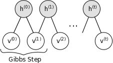
It turns out that the bipartite nature of an RBM means that it is simple to obtain an approximation of the unconditional hidden and visible vectors of an RBM. This can be done using Gibbs Sampling. As a result, when presented with a visible vector, we can get the dependent hidden vector by sampling from the RBM (h0 in the below diagram), and get a less biased hidden and visible vectors by performing several steps of Gibbs Sampling (ht and vt in the below diagram)

Gibbs sampling (image taken from http://deeplearning.net/):

It turns out that we can approximate the Energy function gradient by taking the difference between the outer products of the dependent and independent hidden and visible vectors. Basically, gradient = v0 * h0 - vt * ht. There are I think several ways of looking at this. The first the mathematical justification, which I think isn’t that intuitive (but is rigorous). The other is that if you view each hidden node as a feature detector over the visible nodes. In this case, we want each feature that is activated for a given visible vector to be strengthened for that visible vector, and to be weakened (less likely to activate) for other visible vectors.

There are a few extensions to this basic algorithm for Contrastive Divergence. The first is that it is not necessary to iterate the Gibbs Sampling many times to get a useful measure of the gradient (even iterating only once can give good results). Contrastive Divergence using Gibbs Sampling of k steps is usually referred to as CD-k. The second extension is Persistent CD. This is simply maintaining the state of the hidden and visible vectors of the Gibbs Sampling chain between training examples. This allows faster and better calculation of the unbiased hidden and visible vectors.

Sample Implementation

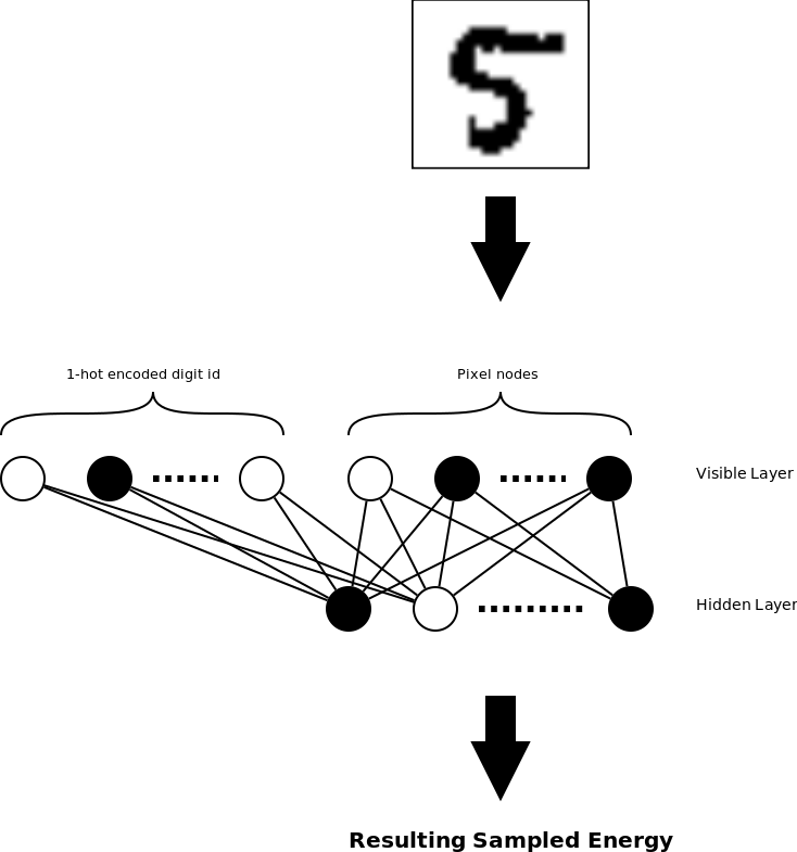
I wanted to build my own implementation of an RBM using Contrastive Divergence for training. While this algorithm is fairly simple, one of my concerns was picking a task where I could easily test that my implementation was working correctly. For discriminative models this is trivial (one can simply examine the classification error on a test dataset), for generative models it is less straight-forward. However, It is possible to use an RBM as a classifier with only a small extension. Say that we want to learn to classify some binary vectors into one of N classes. In this case we could use a visible RBM layer that is the union of the vector to be classifier and a 1-hot class encoding. To classify a given vector, we would try all N possible classification, choosing the one that generates a hidden vector with the least Energy as given by the RBM energy function.

I decided to apply this approach to the venerable task of MNIST digit recognition (using thresholded binary images). In this case the visible layer contains 784 + 10 nodes (784 for the binary image and 10 for the 1-hot encoded digit class), and the hidden layer size is a free parameter (I tried 400 and 800 nodes during testing). After the RBM network is trained, it can be used to classify a given image by choosing the digit classification that results in the minimum energy.

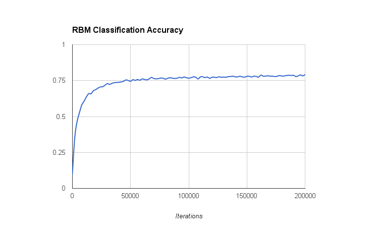
With this system I managed to get up to about 80% accuracy over the MNIST database. This isn’t too bad, I expect this is what a logistic regression classifier (using only the raw pixels as features) would achieve. The graph below shows the RBM classifier accuracy vs iterations (using a batch size of 50).

RBM Extensions

A basic RBM is rather limiting in that it can only deal with binary input vectors. However, there are extensions that allow RBMs to deal with real valued input data (and real-valued hidden layer nodes). Furthermore, it is possible to stack RBMs on top of each other, in effect generating higher level features. In image recognition applications this could be first detecting edges/corners, then detecting lines/circles, then detecting eyes/faces, etc. In this type of application, we could train a series of stacked RBMs, followed by a shallow neural network for image classification. This type of approach is known as a Deep Belief Network, and was the first practical approach to “deep learning” proposed by Geoff Hinton around 2006. One of the advantages of this approach is the RBM layers can be trained using unlabeled data, which is typically much more plentiful than labeled data. Labeled training data would only be needed for the last few discriminative layers.

I won’t explore these extensions for now, as I think this approach to Deep Learning has fallen out of fashion somewhat. When DBNs were originally developed, standard Feed Forward Networks were still largely based on sigmoid activation functions (logistic or tanh), and were trained on CPUs. This made it hard to train deep networks due to the vanishing gradient problem and the comparatively slow hardware. Now, using activation functions such as ReLU, GPUs for greater compute power, and better training algorithms such as Adagrad, we can train deep Feed Forward Networks quite well.

The code for this project can be found on Github: here (warning: code is experimental and may be slightly messy).