In a previous project I experimented with Recurrent Neural Nets (RNNs), their implementation, and application to character-level language modelling. In that instance I used a simple RNN architecture, more or less a standard feed-forward network with an optional recurrent connection between layers. This type of network can learn short term correlations in the input stream, but struggles to learn long-term correlations. To address this problem, a special type of RNN was proposed in 1997, called Long Short-Term Memory (LSTM). This network architecture has more in-built structure, compared to a series of fully-connected layers. I view LSTMs as modelling a “memory latch”. An LSTM cell has one data input, one output, and 3 “control” inputs. The controls can be labelled as input, forget, and read. These affect how the LSTM cell treats the incoming data, the current internal state, and the output of the cell. There are several variations of the architecture of an LSTM cell, a common one is shown below:

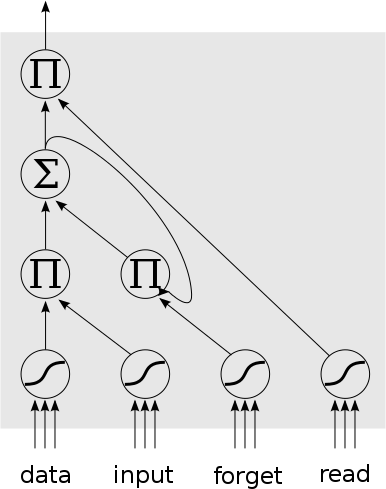
The control inputs are computed by passing the weighted activation through a logistic activation function to restrict the range to 0..1. This then interacts with the data input, internal state, and output via product gates. For example, if the read control activation is close to 1.0, the product with the cell’s internal memory will not change the value, outputting the cell’s memory. However, if the read control is close to 0.0, then it will cancel out the internal state, outputting 0 from the cell.

One thing to point out with an LSTM is that unlike fully-connected layers, not all of the gates have weighted inputs. The inputs of the product gates are not weighted. Only the data and control nodes have weighted inputs, as well as the internal state summation node.

The big advantage of an LSTM is that it can readily store a given piece of input data for many time-steps. All it requires is for the forget control input to be close to 1.0, and for the input control to be close to 0.0. Then the already-contained state will be maintained between subsequent time steps. This storing of internal state over a long term also translates to being able to store the error delta over many time steps. In the case of Back Propagation Through Time (BPTT) over a vanilla RNN, an error delta from time step T has to back-propagate through N time-slices to reach the nodes at time step (T-N). At each time-slice this error delta may be modified and reduced, making learning the weights at time step (T-N) to account for the error delta at time T very difficult and slow. In the case of an LSTM, however, the error delta can be stored implicitly in the LSTM state, in what has been termed an “error carousel”. In short (and putting aside my rather rambling description), an LSTM can learn long-term dependencies far better than a vanilla RNN.

Vectorisation

The previous diagram and explanation of LSTM networks describes a single cell. This is good for understanding the concept, but a proper implementation would need to be vectorised. That is, it would need to deal with “layers” of particular nodes, and connections between these layers would be in the form of matrix transforms. Since I intend to write my own LSTM implementation in the future, I went through the exercise of “unrolling” and “vectorising” the LSTM cell. This is represented in the below diagram.

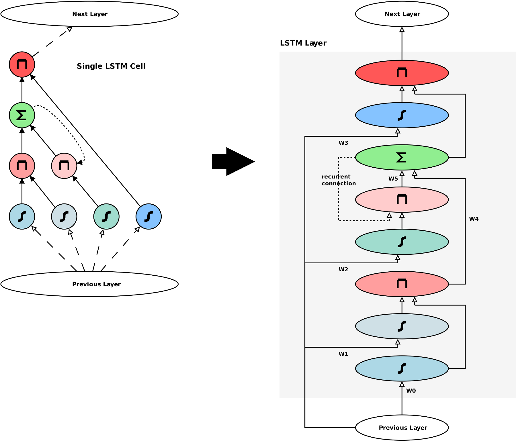
In this diagram, the right-hand-side illustrates an LSTM Layer, that can consist of a parametrisable number of LSTM cells. In this layout, there are 6 weighted connections, each associated with a weights matrix. In this case matrices W0, W1, W2, and W3 are of size (prev layer width x LSTM width). The matrices W4 and W5 are of size (LSTM width x LSTM width). The Product Layers are different compared to other layers (such as Logistic layers), in that they do not take a weighted sum of the inputs and then perform an activation function. Instead, the Product Layers perform a Hadamard product of the two incoming matrices. The inputs to the Product Layers are unweighted. Another special aspect of the Product Layers is the way their derivative is computed, to then back-propagate the error delta through the network. The error delta is back-propagated along each of the two incoming connections of a Product Layer, component-wise multiplied by the input along the other connection.

In the future I plan to implement a stand-alone LSTM network using CUDA. This will give me a better grasp of the nitty-gritty details. But for now, I chose to take the quick and easy path of using Tensor Flow to play around with LSTMs.

Character Level Modeling

In my previous look at RNNs I applied them to the task of character-level language modelling. Specifically, I trained an RNN to predict the next character in a sequence, and then I sampled from this network to generate new text. If such a network is trained on say, the works of Shakespeare, then the text it generates will have a “Shakespearean” quality to it. This is a fairly simple task, but has the advantages that training data is easily available, and it is straightforward to judge whether the RNN is doing the right thing (if it produces garbage text, then something is obviously wrong). For trying out LSTMs I decided to use the Tensor Flow framework, rather than writing my own implementation. I intend to do that later, but for now this is a quick and easy way of playing around with LSTMs, and has the added benefit of giving me more practice with the TensorFlow API. Below is a snippet of text generated by sampling from the character probabilities of an RNN using LSTM layers, trained on the works of Shakespeare for 100,000 iterations. I used a batch size of 32, a time-step horizon of 32 for the BPTT algorithm, the network had 2 layers of 128 LSTM cells, bracketed on either side by fully connected ELU layers of 128 nodes.

the house of after your death. god and you think of you in pride when we are more remember out a better work save men of their peers at the form where i may be longer than you to the queen the one the lion it will speak. for the cardinal the general fortune hath refus’d me to your wify. somerset. what’s your window?’ and let it be so! for the business! petruchio. as the fair fast people’s page is not an excellent accent that thou wilt and in the boy love indeed about what we are not alive leave the other and sword the curtain and the hart and this that should be. beat. sir john of lancaster i did not and more than the fear of god?

Compare this snipped with the text generated by my standard fully connected RNN in my previous project:

i do now stood i’ tear and kneel my earth and tall so; you meather i would come whom the world you sir. exeunt. others phaketh should those harryworn and but lartius. rom. i am drunk’st if you do and will coriolanus. where heaven deserve or loving of his percy done at this scene in himself bears to kiss is true apollaysarty and in a pluckedner’s grosser for him. fair gentleman. and ancient slodky deny so forswey heaven: elsewis.

It can be seen that the LSTM version produced more coherent text.

Variants and Future Work

Having discussed LSTMs, it is worth noting that there are several variations and alternative approaches that share a common theme. A relatively popular one is the Gated Recurrent Unit (GRU), which has one less control input (thus it is easier to train, in theory) than the LSTM but appears to retain a similar performance level. In addition to these variations of what I’d call a “differentiable latch”, there is also work on creating neural networks that simulate higher level data structures. A “differentiable stack” has been developed, along with a “differentiable turing machine”. This looks to be a promising area of research that could lead to neural networks that can learn to perform quite complex tasks.

In terms of future work for me, I’ve played around with LSTMs using the TensorFlow framework, but I intend to create my own CUDA implementation in the near future and apply these to some interesting Reinforcement Learning tasks.

The code for this project can be found on Github: here (warning: code is experimental and may be slightly messy).