In this entry I’m going to describe a method for Robot Localisation that I implemented/developed during my time working on Robocup in 2006 and 2014. It will be super high level, but the nitty details are available in my undergraduate thesis.

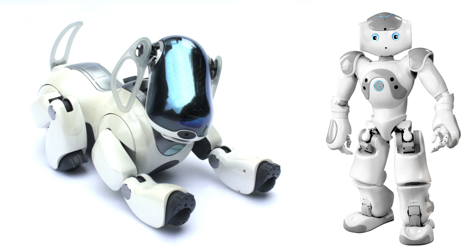
Way back in 2006 (and more recently in 2014) I was part of the UNSW Robocup team (rUNSWift), a team of undergraduate thesis students participating in an international robot soccer competition. This involved programming autonomous robots (Sony AIBOs in 2006 and Aldebaran Naos in 2014) to play soccer on a miniature field. One of the key components of such a system is localisation, or more generally: state tracking. This basically translates into solving a Partially Observable Markov Decision Process, where the inputs are observations (through the robot’s camera) of various landmarks, as well as process inputs in the form of odometry data. The goal is to use these inputs to determine quickly and accurately the current state of the world (ie: the robot’s position, the ball’s position and velocity, etc). The main difficulty of this problem is being resilient to observation and process noise/measurement errors, as well as things like falling over or being moved by a referee. One additional constraint is the comparatively weak processing power available on the platform (all processing must be done on the robots, which I think had something like a 500mhz MIPS processor on the Aibos, and a 1GHz Geode on the Naos).

In 2006 there were really two dominant approaches to this problem, at least in our league. The approach used by rUNSWift was based around the Kalman Filter (and to the best of my knowledge several other teams such as Newcastle University which ended up winning the competition that year). An alternate approach used by many teams was based on Particle Filters (used by the German Team and many others). I won’t really talk much about Particle Filters (also more generally known as Monte-Carlo Localisation), other than to mention their main advantage is being able to handle arbitrary probability density functions and non-Gaussian noise models. Their main disadvantage (in my opinion) is their computational cost and poor scaling with the number of state dimensions.

Kalman Filter

The Kalman Filter is an algorithm that integrates noisy measurements over time and estimates a joint probability distribution over the target variables. I think an easy-to-understand way of looking at it is as a sophisticated running average. Say we want to estimate the value of a single variables, but the measurements we receive are noisy. The simplest way to do this is to simply compute a weighted running average:

cur_estimate = 0.1 * measurement + 0.9 * cur_estimate

A Kalman Filter is in some ways a more sophisticated running average. The sophistication comes from the fact that the Kalman Filter dynamically weights the measurements and the current estimate based on their relative certainties, can effectively handle multi-dimensional states/measurements that have correlations, and incorporates a process update step.

I wont go into the derivation nor the equations involved in performing the measurement and update steps, but I’ll specify the “interface”. For an N-dimensional filter (if we are tracking a robots x,y position it would correspond to a 2-dimensional filter), we always have an N-dimensional state vector, and an NxN covariance matrix. The covariance matrix is a representation of the uncertainty of the state vector, additionally encoding the correlations between the dimension in the non-diagonal elements. These are updated in the measurement and the process steps. The measurement step always reduces the uncertainty, while the process step always increases it. The inputs of the measurement step are the observation vector, a matrix that maps the state vector into observation space, and a vector representing the uncertainty of each dimension of the measurement. These are combined with the current state and covariance matrix to output the new state and covariance. The inputs to the process update step are the change in the state vector, and the change in the certainty of each element of the state vector. Again, these are combined with the current state and covariance matrix to generate a new state and covariance. Examples of a “process update” are odometry measurements, or open-loop motion commands.

This basic Kalman Filter is useful in many applications as a way of dealing with noisy measurements and processes. However, in its current form as described above, it is not useful for Robot localisation. This has to do with the nature of typical state observations. The standard Kalman Filter expects the mapping between observation space and state space to be linear. When this assumption is violated, we must use an Extended Kalman Filter.

Extended Kalman Filter

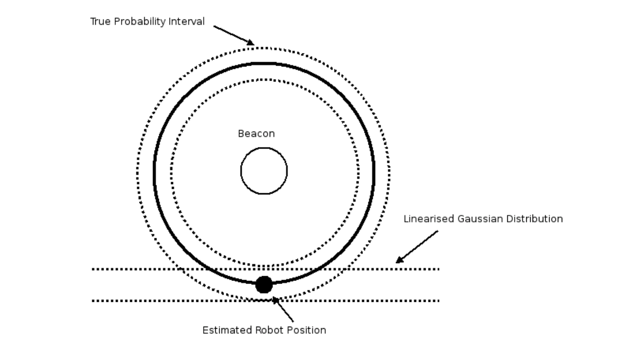
The Extended Kalman Filter is a relatively minor modification to the standard Kalman Filter that allows it to handle non-linear mappings between observation and state space. The main idea is to approximate the non-linear mapping with a linear one. This is done by taking the derivative of the function that maps observations to state space at the current state vector. This is known as a Jacobian matrix. This matrix effectively becomes a linear approximation of the non-linear function. This concept is shown in the diagram below, with the example observation being a distance measurement to a fixed beacon landmark. In this case, the mapping function between state-space (x,y position) and observation looks like a circle. However, when this is linearised around the current estimated pose, it is a tangent at the current estimate.

The calculation of the Jacobian will depend on the type of observation for the current measurement, and the specific equations that map the tracked state to the observation dimensions (it is simply a matrix of partial derivatives). However, once the Jacobian is available, it is a very straight-forward plug-in to the standard Kalman Filter equations.

One problems with the Extended Kalman filter is that the linearisation process is “lossy”, and as a result we lose the optimality guarantees of the standard Kalman Filter. The standard filter is a provably optimal filter in the case of a Gaussian noise distribution of the measurements and process updates. However, even under these assumptions the Extended Kalman filter is no longer “provably optimal” due to the linearisation process.

Multi-Modal Filter

The Extended Kalman Filter as described above was the basis of the rUNSWift localisation system in 2003. A separate filter was used to track the robots pose (x,y,theta), and the ball’s position. One of the problems with this filter is it is single-modal. The state of the filter is represented by a single state vector and covariance matrix. As a result, it cannot accurately model multi-modal probability density function (PDF), nor can it deal with observations that are inherently multi-modal (eg: observing a non-unique or ambiguous landmark). The solution is to alter the Extended Kalman Filter, going from a single Gaussian representation of the state estimate to a weighted sum of Gaussians representation. This approach can more accurately model a wider class of PDFs, handle multi-modal observations, and handle spurious observations (observations that don’t fit the expected error model).

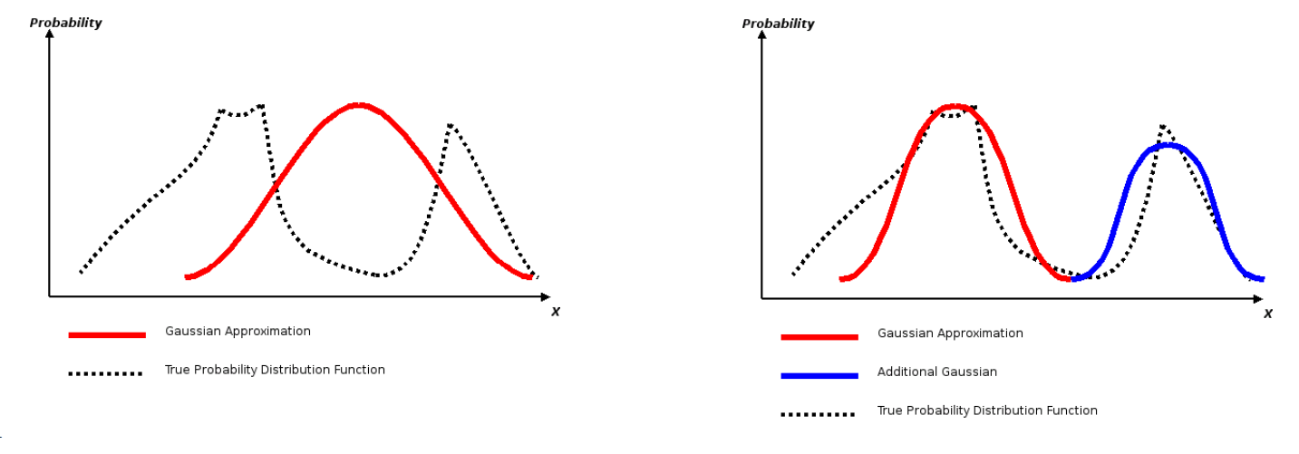
To handle a multi-modal representation we do not need to change the EKF very much. At its core, we simply treat it is N separate EKFs, where N is the number of modes we are using. Each mode has a mean state vector, a covariance matrix, and a weight. The weight represents the confidence that the corresponding mode is the true distribution. When performing a measurement update, each mode is updated as in a normal EKF independently, with each weight updated according to how well the current observation matches the mode’s hypothesis. Once every mode is updated, the weights are renormalised so that they sum to 1.0. A typical approach is to then use the top-weighted mode as the best estimation of the system state.

Having multiple modes as part of the density function is extremely useful for several use cases. The first is filtering out spurious observations. A standard EKF is good at dealing with noise that is Gaussian in nature. However, spurious noise (eg: observing a landmark by misclassifying cluttered background) is handled far worse. One way to handle this is for each observation we clone each mode, and apply the observation to only one of the pair. The other mode has its weight scaled down by a factor proportional to the expected rate of spurious observations. This way we can keep two hypotheses in each case, one where we treat the measurement as legitimate, and another where it is treated as spurious. Either the immediate weighting between the two, or later observations, will determine which is correct. The other benefit of a multi-modal distribution is being able to handle ambiguous observations. If a robot observes a non-unique landmark, it cannot know from the measurement alone which actual landmark it is. For example, in the 2014 SPL league the goals (a very useful landmark) are the same colour on both sides of the field. As a result, a goal post observation does not contain information about which actual goal post is it, with there being 4 possibilities. We can instead treat an ambiguous observation as N possible uni-modal observations. We then copy every existing mode N times, and to each apply the uni-modal observation. The subsequent observations and relative weights will determine which hypothesis was correct.

One of the tricky bits of a multi-modal filter is merging modes. For many observations we multiplicatively generate new ones (doubling or tripling or more the number of modes). This would quickly result in more modes than can be computationally handled. For this reason (and a few others), we need to merge modes that are very similar to each other (similar state vectors and covariance matrices). There are probably a few viable ways of doing this, but we used to simply do a weighted sum of the two modes if each element of their state vector and covariance matrix were within some epsilon threshold.

Distributed Filter

The main innovation that came out of my work in 2006 on the localisation system was to make it distributed across the entire team of robots (in 2006 each team consisted of 4 robots, in 2014 it was 5 per side). The idea was that instead of each robot independently tracking a 7 dimensional state (3 for the robot pose, and 4 for the ball position and velocity), they would instead track a 16 dimensional state (19 dimensions in 2014 due to the extra robot). This corresponds to 12 dimensions for the poses of each robot on the team, and 4 for the ball. Each robot would update only the dimensions that corresponded to its pose and the ball. However, each robot would also transmit its observations to its teammates, which could then incorporate these into their own filters, updating the poses of their teammates in their filter. On the surface this may not have much benefit, until you consider that the ball is a common “landmark” that can be seen by multiple robots on the team. With the way that this scheme affects the correlations in the covariance matrix, the end effect is that the ball becomes a sort of moving landmark that can be used by the robots to localise from. In the non-distributed filter, when a robot observes the ball it does not carry any information about the robot’s pose, since it is not a fixed landmark. However, in the distributed filter, the ball’s position variance can be lower than the robots own pose variance due to teammate observations. As a result, when it observes the ball, it can actually localise it’s own pose. This had pretty significant implications for gameplay, since it is often the case that the robot kicking the ball does not see any other landmarks (as it is focused on the ball), whereas its teammates have a wider view of the field.

This is a fairly good video from 2006 where one of our robots is able to score extremely quickly, partially due to it’s excellent and fast localisation:

Domain Specific Issues

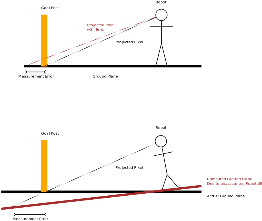
So the algorithm/approach described so far is relatively straight forward, and actually fairly simple to implement. However, when applied to the Robocup domain, many issues come up when the assumptions of the algorithm are violated. The worst offender is probably the non-Gaussian nature of the noise in the measurements. The issue in 2014 that probably caused me the biggest headache is distance measurements to various landmarks. In this case the robot is a bipedal Nao that has a camera in its chin (so quite high in the kinematics chain from the ground). When the robot detects say a goal post in the image, it calculated the distance by projecting a “pixel ray” through the bottom-most “goal pixel” in the image, and intersecting this ray with the ground plane. This is then used to calculate the distance of the goal from the robot. In this case problems arise when the goal-post is far away, and hence near the horizon in the camera image. In this case, a small pixel error (in terms of detecting the bottom of the post) can result in a very large (and non-symmetric) error in the measured distance. A similar problem arises when the ground plane is incorrectly calculated. This can occur when the bipedal Nao robot sways in an unpredictable and undetectable way. In this case, the kinematics calculations may yield an incorrect ground plane, which in turn results in an error in the distance calculation when the pixel ray is intersected with the ground plane. Both of these scenarios are shown in the diagram below:

I wont go into detail on how these types of issues were address, and in fact I could go on for a very long time about the numerous cases in Robocup where the basic assumptions of the Kalman Filter are violated, and all of the time consuming (to develop) “hacks” and workarounds that were developed to address them. However, I might leave that for a later writeup. For now, here is a video of our semi-final game against the 2nd best team in 2014, B-Human. It was probably the best match of the tournament.