Using Neural Networks for agent control and game playing is a very interesting area. In previous projects I’ve used the DQN algorithm to play connect-four, and later a Recurrent Neural Network (RNN) to control an inverted pendulum balancing agent. I think that using RNNs to control agents is a very interesting area of research, since in this case the network can implicitly learn its own suitable state representation and update method for Partially Observable Markov Decision Processes (POMDPs). I had some success training an RNN for a fairly straight-forward task (inverted pendulum), so now I wanted to try something more complex. In this case I chose the task of controlling a “hovercraft” (so a nonholonomic system) on a 2D track. I wanted to implement the decision process using an RNN, taking as input only the raw instantaneous simulated sensor data. To make the problem more complex/interesting, the sensor data is in the form of a 1D “stereo” camera on the front of the simulated hovercraft. This means that the RNN has to first correlate the two 1D images to extract the depth information, keep track of this state from frame to frame to determine its current velocity and other necessary derived state data, as well as learn the correct control policy. While at first glance this toy task looks fairly similar to the numerous other examples that can be found online, it is in fact much harder. The existing examples I’ve seen all seem to use a “sonar” type simulated sensor, and make variables like the velocity of the agent directly available to the policy function. This initial description of the problem isn’t super detailed (more detail below), so I made a quick video of this environment (in this case I am manually controlling the hovercraft):

World Simulation and Control Task

In this toy task, the world consists of a controllable “hovercraft” vehicle, and a static 2D track. The hovercraft has 2 control inputs, turn and accelerate, both of which have 3 possible values (1.0, -1.0, 0.0), corresponding to turning left or right, and accelerating forward or backward. The acceleration is performed in the direction that the hovercraft is facing, which is distinct from the current velocity direction. When the hovercraft makes contact with the track wall, it bounces off in an elastic collision, with the velocity magnitude decaying a significant amount.

The track itself is a circuit with a varying width. There are a number of ways I could have gone about procedurally generating the track, or even manually design my own tracks. In the end I decided to go with a quick and simple implementation where I start off with a circular track and then randomly radially perturb each vertex. The magnitude of the perturbations is sampled from a uniform random distribution, with the magnitude inversely proportional to the frequency. Basically this means that you get a track with many small deviations, and a few larger ones. I could have gone with something like Perlin Noise here, but I didn’t want to spend too much time on the track generation part of the project.

The above algorithm generates the track skeleton, then to generate the actual track walls I simply offset inward and outward from the skeleton by a width amount, which is sampled from a uniform random distribution. One important detail to note here is that the walls of the track are randomly coloured. This is important for the sensors, discussed next.

Sensors

One of the main aspects I wanted to explore is a relatively complex observation of the environment as input to the policy function. I decided that the agent should sense the environment through a 1D stereo “camera”. Basically this is implemented as two cones of sample rays emanating from the “hovercraft” into the environment. The colour of the track wall at the intersection point of each ray is the sensed “pixel” colour. Since the two cones are separated by some baseline distance, they would sense slightly different 1D images of the track, and this difference can be used to determine the distance to the track wall (stereopsis). At least that was the theory. The diagram below shows a schematic of how the 1D “stereo camera” senses the world and converts this to two 1D arrays of pixel colors.

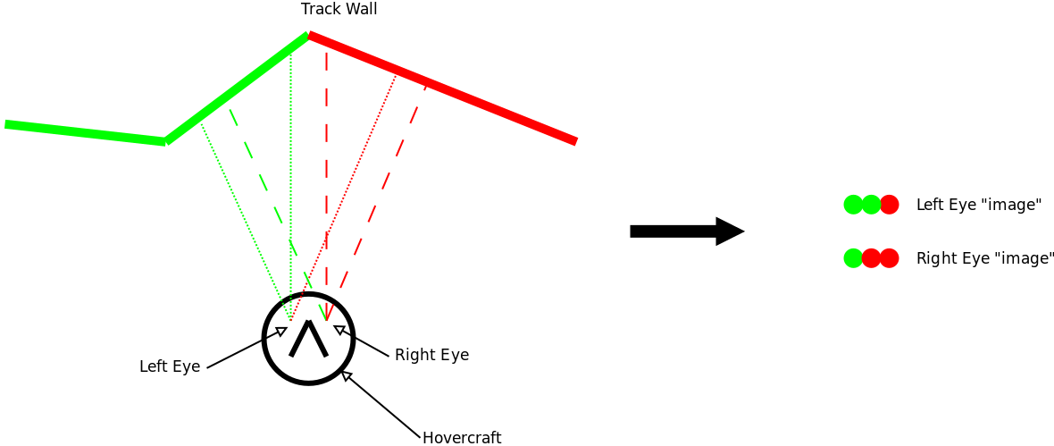
Given the fact that I wanted the agent to sense the world using stereo correlation to determine the distance to the walls, this meant that the walls had to be non-uniformly coloured. If say the walls were just flat white, then you cannot really determine the distance. For this reason I made the walls have a randomly assigned colour that smoothly changes along the wall segments.

Reward and Learning Setup

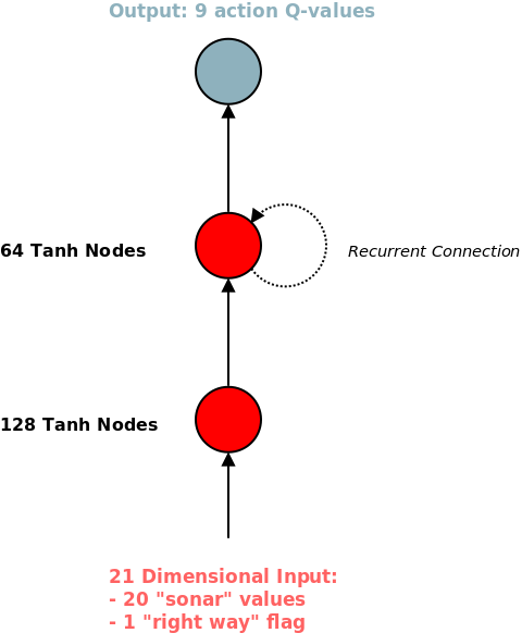
The overall aim is to train an agent that can traverse the track as quickly as possible. This leads to a fairly natural reward function, at every time step the reward is equal to the amount of the track traversed since the last time step. This is measured simply by projecting the current hovercraft’s (x,y) position onto the track skeleton. The learning setup is almost identical to that used in the inverted pendulum balancing task. A simple RNN is used, with a tanh activation function for the hidden layers and a linear output layer. The inputs are raw observed pixels of the two RGB “stereo cameras”, which results in an input dimension of 6 * NUM_PIXELS_PER_CAMERA. The output is 9 dimensional, each corresponding to the Q-value of the corresponding action. The learning method is based on the DQN algorithm, adjusted slightly for an RNN.

The Problem Solving Begins

Ideally the approach described above would “just work”, but there would be little fun in that. The first few training attempts ended in miserable failure. The resulting agent appeared to be unintelligent, either performing what looked like random actions, or sometimes just running into a wall and then not doing anything. I realised relatively quickly that one thing missing from the agent’s inputs was any kind of indication of track direction. If the walls are randomly coloured, even if the RNN can learn to extract depth information, there is no indication of whether going “forward” would result in a positive or negative reward. This apparently random reward behaviour (from the agent’s point of view) makes useful training impossible.

I tried several ways of indicating track direction. The first attempt was to give the walls a fixed colour pattern, rather than random. The theory was that the agent could learn what the track looked like in the forward and backward directions. This didn’t work so well. I think the reason is that, despite the colour pattern of the walls being fixed, it was still a fairly complicated signal to learn which way was “forward”. The RNN would basically need to memorise the track’s appearance.

The next modification I tried was to treat the progress along the track as one of the RNN inputs. So one of the input dimensions is the current 1D track position of the hovercraft. The idea here was the RNN could learn that as this value increases, it is going “forward”. This sort of worked, in that it resulted in slightly better behaviour, but was still far from acceptable.

At this point I had two theories, either this task was much more complex than I initially considered, or there was a bug in my code. I decided to go back to basics and simply give enough input into the network that it would be able to learn a good policy, and work backward from there. I decided to scrap the “stereo camera” idea for now, and replace it with a “sonar”. Meaning the agent receives a number of distance samples in a frontal arc, so it could know when it is about to hit a wall, etc. To make the learning task even easier, I provide the forward direction of the track relative to the current facing direction, as well as the current relative velocity of the hovercraft. With these simplifications the RNN was able to learn a decent policy. This was encouraging and I could work from this baseline to determine what exactly was causing the poor performance on the original task formulation.

At some point I realised that a good way of signalling the track direction is to simply provide a boolean flag as an input that indicates whether the hovercraft is facing the wrong way. Basically, this input is 1 if the heading is within 90 degrees of forward, and otherwise -1. Think of it as a “WRONG WAY” sign (may have seen it in some arcade racing games). By introducing this flag, I was able to remove all the other hint inputs, with only the sonar sensor values remaining. I think this is an ok setup, with the RNN inputs being fairly realistic and not too synthesised from external knowledge.

So in the end, the inputs to the network are 16 dimensional, with 15 of these corresponding to sonar depth values sensed in a cone in front of the hovercraft, and 1 corresponding to the WRONG WAY flag. The final result of this process is I was able to train an RNN to control the hovercraft in a fairly reasonable way:

It should be noticeable that the agent is often wiggling left and right. I think this is to get a wider view of the area in front of it, as the simulated sonar sensor only has a “field of view” of 120 degrees. I think the wiggling behaviour is pretty cool anyway.

I should point out that training the RNN seemed to be a fairly fragile process, certain hyper-parameter combinations resulted in a network that could reasonably control the hovercraft, but would also get into some problems. I found that adding more layers would often lead to worse performance, even if training was run for a longer time. This can be seen in the video below, where at some point the agent gets turned around and gets confused, as well as getting stuck on walls.

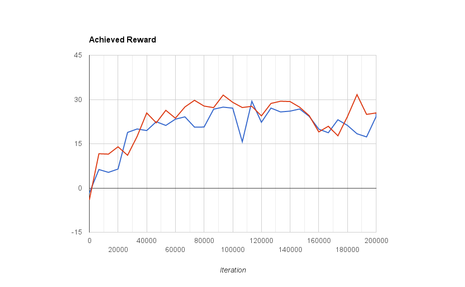
In addition to simply visually inspecting the quality of the hovercraft control, below is a graph of the average reward gained by the RNN controlled agent as a function of the learning iterations. I only plot two learning runs, so not really a rigorous analysis, but it demonstrates that training RNNs with Reinforcement Learning can result (in this case at least) in some interesting performance dips. It isn’t a nice monotonically increasing performance curve.

Lessons Learned and Future Work

I learned a few lessons during this project. Basically I learned that Recurrent Neural Networks are hard, and training them for Q-function approximation is hard. It seems that simply adapting the DQN algorithm for RNNs doesn’t result in stable learning on any kind of complex tasks. I was able to arrive at an acceptable policy when using sonar input, but using the more complex 1D stereo image input totally failed. Even the sonar input was difficult to train, with some otherwise reasonable hyper-parameters causing weird instabilities. I’d definitely like to refine my approach in the future and come back to this task, controlling the hovercraft using the stereo vision data as input.

There are several obvious areas to explore:

• control the magnitude of the RNN gradient,
• use an LSTM or other similar memory gate, instead of the fully connected recurrent layers,
• look at tweaks to the DQN algorithm to stabilise the learning,
• try different Reinforcement Learning techniques such as SARSA or TD-Learning
• consider Policy Gradient methods.

There is enough here for some interesting future projects and improvements to this work. Stay tuned.

The code for this project can be found on Github: here (warning: code is experimental and may be slightly messy).