So in the previous part I described the very simple first attempt at using neural nets to perform handwritten digit recognition. In this part (in no particular order) I’ll describe some of the variations I tried, improvements I discovered, and lessons learned.

Tanh Activation Function

In the first few versions of the code, I was using the logistic function as the hidden (and output) layer activation function. This turns out is far from optimal. The hyperbolic tangent (or tanh) function is another function that has a “sigmoid” shape, but turns out to have nicer properties when it comes to backpropagating a loss gradient through a feed-forward neural net. One of the reasons is that it tends to have a larger gradient as compared to the logistic function (1-x*x vs x - x*x where x is the value of the function). Switching to the tanh function improved the performance of the neural net by good amount.

Softmax Output Layer

Initially I used the logistic function (outputting values in the range [0..1]) in the output layer, and would take the largest activation value of the 10 nodes as the result digit. This works ok, but is not strictly speaking the right way to approach this problem. The task is classifying an image into 1 of 10 classes. What we really want as the output is a probability distribution across the 10 classes, which a logistic output layer does not give you. The Softmax function is actually what we want in the output layer in this instance. This has two benefits, one is that the output can be interpreted as a proper probability distribution (which may be useful downstream in a wider system), and two is that the gradient signal from the loss function is much better, resulting in faster training of the network. Switching to a softmax output layer resulted in about 0.3% reduction in the error rate (which was about a 20-30% relative improvement), but more importantly a much faster training time.

Gradient Descent Policy

In the initial versions of my neural network I was using a “hand rolled” gradient descent policy, using a mix of things like Nesterov momentum, per-weight learning rate scaling, adaptive global learning rate, etc. This wasn’t such a great idea in retrospect as I ended up wasting a fair bit of time tweaking various parameters, having the learning rate too high and blowing out the weight updates, or too low and taking too long, etc. At some point I grew frustrated and implemented the Adam algorithm, which comes with a nice set of “recommended” parameters and this ended up working very well.

Dropout Regularization

Regularization refers to the measures taken to prevent a classifier from over-fitting the training dataset and performing poorly as a result on the test set. I found that my network was suffering from over-fitting in some instances as it ran past a threshold number of iterations of gradient descent. Common solutions include L1 and L2 regularization, which put a cost on the magnitude of the weights. A more recent method specific to neural networks is dropout regularization which basically makes every node during training behave stochastically. During training, every node will be “turned off” with some probability, which discourages co-dependence between different signals, and simulates an ensemble of classifiers. This actually turned out to be both very simple to implement and very effective. It is important to note that during testing of the network, the nodes are not dropped out.

Autoencoder Pre-training

One of the problems with neural networks with several hidden layers is that, although its representative power increases, it becomes harder to train. One of the proposed solutions to this is to start the gradient descent training from a good starting point, as opposed to simply using randomly initialised weights. One idea is to pre-train individual hidden layers as autoencoders.

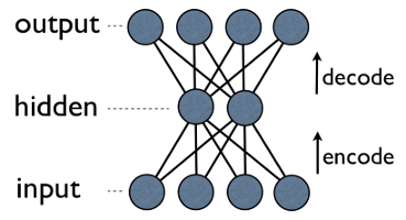
An autoencoder is a type of feed-forward neural net that has an output layer with the same dimensionality as the input, and its target output is equal to the input. Autoencoders can be used to extract some higher level features from an input signal, and perform dimensionality reduction while retaining as much important information as possible. One variant is the de-noising autoencoder, in which cases we stochastically dropout parts of the input signal at training time, but use the unaltered input in the loss function. In the specific case of digit recognition, we could set some random set of pixels of each training image to 0, but then expect the autoencoder to output the original image. Theoretically pre-training each hidden layer of a feed-forward network as the hidden layer of a de-noising autoencoder could help get a good initial state for more effective training using gradient descent.

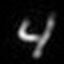
Below is an example of the performance of a trained autoencoder with a single hidden layer. Around 0.35 of the input pixels are dropped during training, and the hidden layer is half the size of the input layer. As can be seen, the network does a good job of reconstructing the input despite the dropped information and layer bottleneck.

Generating Training Data

Having lots of training data is good, but is not always possible. In the MNIST dataset we have 60,000 training samples, and 10,000 test samples. For a moderately sized neural network this is not that much training data. Fortunately, we can fairly easily generate new training data from the existing images. If we assume that rotating a digit image by up to +-10 degrees and translating by up to 10% of the image size does not change the fundamental “appearance” of the digit (ie: what digit it should be recognised as), then we can generate loads of new training data. I used the OpenCV image library for convenience, and I ended up generating 5 additional random images for each baseline training image using small random rotations and translations. This yields a total of 300,000 training images, which ends up helping the accuracy of the trained neural network significantly. There are other more complex transformations that I could have used (eg: elastic distortions), but I couldn’t be bothered :-)

End Result

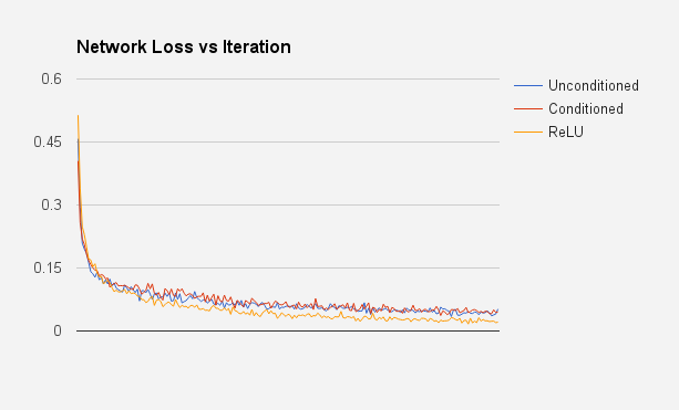
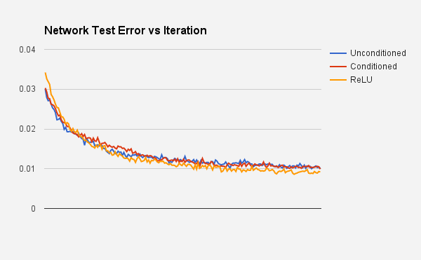
So the end result of trying several of the above mentioned improvements was both surprising and satisfying. It was surprising because using a denoising autoencoder pre-training step did not really improve the accuracy of the final neural network when using the tanh activation function (but it did help when using the logistic function). Having said that, the ReLU function network ended up working the best (with no pre-training). Below are the results for the three different approches, showing the network loss vs time, and network performance on the test dataset vs time. I truncated the first few iterations for the test error graph to better show the relative performance of the approaches (otherwise the difference gets lost due to scaling of the y-axis). The headline error rate achieved is 0.9% by the Rectified Linear Unit network, with a 784 -> 784 -> 392 -> 196 -> 10 network (3 hidden layers). The other networks (tanh activation with and without autoencoder pre-training) achieved slightly higher error rates, but still under 1%.

The code for this can be found on GitHub

Summary of lessons learned

• Choice of activation function matters greatly;
• Softmax output is better than logistic for this class of problem;
• Autoencoders are neat, but don’t provide much benefit for pre-training the network;
• Deep ReLU networks are possible to train with a good learning policy;
• Dropout regularization works great at avoiding overfitting;
• Having good learning data and lots of it is important;
• It turns out pre-training to handle deep networks is no longer considered necessary. The ReLU function which doesn’t suffer from vanishing gradient so much and improved descent algorithms seem to make deep nets tractable.

I think I’m going to leave this problem alone for a little while, but will come back to it when I look into Deep Belief Networks and RBMs.

The code for this can be found on GitHub: here (warning: code is experimental and may be slightly messy).