After implementing a simple Recurrent Neural Network (RNN) for character-level language modelling, the natural next step is to port this implementation to CUDA. RNNs typically take a long time to train, so using the computational power of GPUs is definitely a good idea. I have already developed a CUDA based Feed-Forward Neural Network (FFNN) implementation (as well as several variants), so I could re-use a lot of those foundations. One of the interesting aspects of a RNN is that it offers the opportunity to meaningfully exploit stream level parallelism from CUDA. For FFNNs there isn’t too much to be gained from using parallel streams, as the back-propagation algorithm is mostly sequentially dependent (there is two-way parallelism available in the backprop stage, but it’s not much). This available parallelism meant I had to structure my code a bit better and provide more abstraction than my FFNN CUDA implementations. In this “blog” entry I’ll describe the details of this implementation and several performance related tidbits.

Implementation Overview

As I mentioned above, this implementation heavily draws on the foundations developed in my FFNN implementation. The main difference is the expansion of both the forward and back-propagation stages over the unrolled RNN. This requires a lot more buffer memory to hold the inputs/outputs of each layer and the layer deltas. If the network is unrolled for N steps, then the memory required for each of these buffers will go up by a factor of N. Another difference is the need to zero out these buffers. Depending on the particular layout of a network, the layer inputs and deltas may be incremented multiple times during a forward/backward pass, once for each corresponding connection. This is compared to say a normal FFNN where each layer only has a single input and output connection. Another significant difference to the CUDA FFNN implementation is that I wanted to support stream-level parallelism. To do this I decided to add a layer of abstraction between the neural network logic and the CUDA low-level implementation. I did this by inserting an intermediate TaskExecutor which could be invoked to perform various operations such as matrix multiplication, activation functions, etc. The idea was to have multiple CPU threads performing the NN logic, each with their own TaskExecutor, which in turn operated in its own CUDA stream. All of the synchronisation and logic would be performed in the NN logic layer, with the TaskExecutors being shielded from the details of synchronisation.

Performance Issues

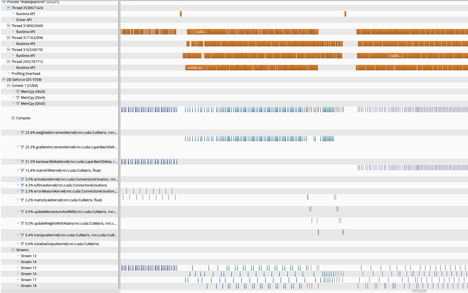
After the finishing the first version of the system, I found that the performance was mediocre. The CUDA based implementation was only a little faster than my CPU implementation. This was in stark contrast to my experience with FFNNs where my CUDA implementation was around 40-50x faster. So naturally the first port of call in this situation is to profile the code. NVProf is a very nice profiler and visualiser for analysing CUDA applications. A quick glance showed that my code wasn’t spending nearly enough time actually computing things, but instead was stalled on things like API overhead (see below for an NVProf graph of the runtime performance). To address the performance problems I decided to make use of both stream level parallelism, as well as a few tricks to reduce overhead.

Shared Buffers

In the initial implementation I allocated a separate memory buffer for every per-slice element. This includes the delta accumulation buffers and incoming activations for each layer. These buffers accumulate values and must be reset to 0 after every training batch is processed. Setting a buffer to 0 takes an epsilon amount of time, but incurs some API call overhead. When the trace length of the RNN training is increased, it also increases the number of buffers that need to be cleared. A better approach is to have a single buffer across the entire trace, with each slice being an index into this large buffer. The advantage here is that this large buffer can be set to 0 in a single call, avoiding the overhead from numerous API calls to clear many smaller buffers.

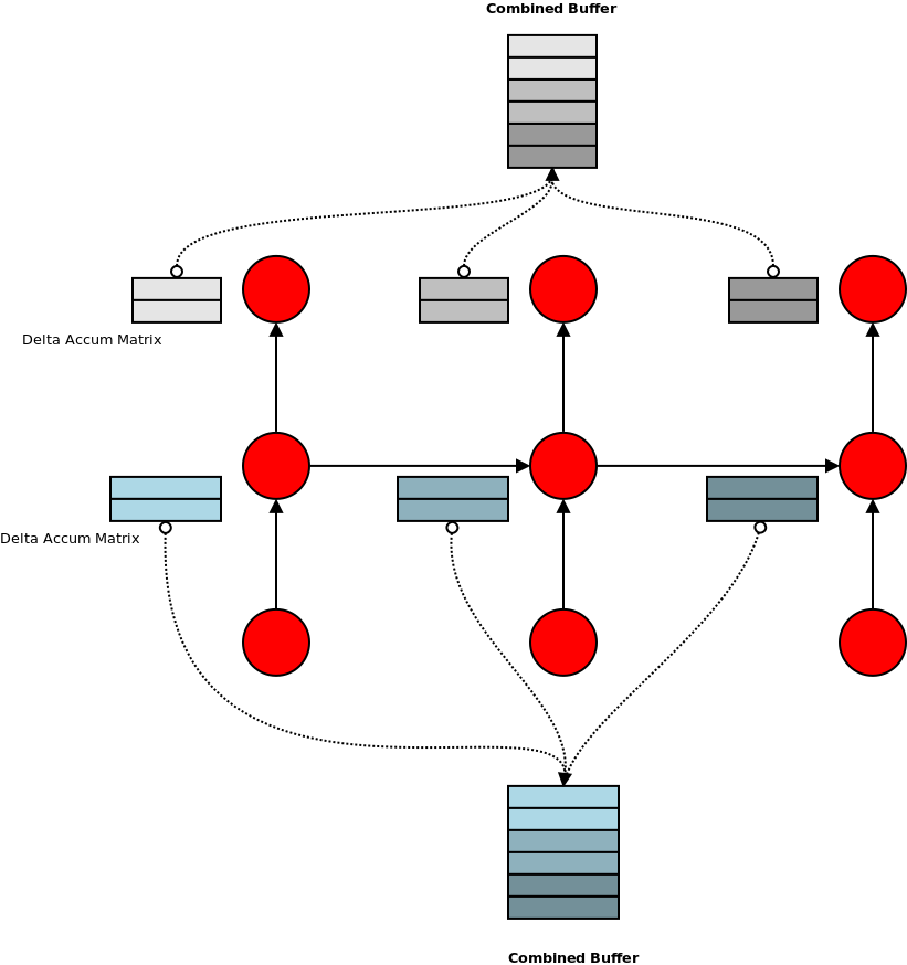
A similar trick can be used to improve the utilisation of bandwidth between system RAM and GPU memory. Each training iteration involves transferring N input batches and N output batches to GPU memory, where N is the trace length. Naively this would be implemented as 2N calls to memcpy. However, if we use a single buffer for the N inputs and another for the N outputs, we can do this in only 2 calls. This results in a much better use of the available bandwidth as a single large memcpy is more efficient than many small copies.

Double Buffered Training Data

While on the topic of the optimal use of memory bandwidth, double buffering can be used to overlap the processing of the current training batch with the uploading to GPU memory of the next batch. Instead of having a single buffer for sample network inputs/outputs, we have two: a “front” and a “back” buffer. Each training iteration we assume that the “front” buffer already has our training data and can start the processing to calculate the weights gradient straight away. In the meantime, we asynchronously start a copy of the next training batch into the “back” buffer. At the conclusion of the processing of the “front” buffer, the “back” buffer should have finished copying (if not then block until it does), and we can simply swap the buffers and continue to the next training example. In this way the cost of the memcpy is (ideally) completely hidden, as it is performed in parallel with the computation.

Stream Parallelism

The final piece of performance enhancement that I tried was stream level parallelism. This basically means running more than one stream of computation in parallel on the GPU. This is useful to do if a particular stream is blocked on something (API overhead, memcpy, etc), or if the GPU has spare resources in cases when a kernel does not have sufficient degree of concurrency to occupy all the Stream Processors. In these cases the GPU scheduler can either switch to running a kernel from a different stream, or it can run multiple kernels concurrently.

Using stream level parallelism at the low level is not difficult, it simply requires passing in an extra “stream_id” parameter to kernel invocations and memcpy operations. However, I found it best to abstract that away from the “logic” code a little, using a TaskExecutor abstraction for the CUDA tasks. Each executor would have its own stream, and be used by its own CPU thread.

There are a few bits of available stream parallelism in the RNN Back-Propagation Through Time algorithm, some being more complicated to implement than others. These are in order of difficulty:

1. resetting of the accumulation buffers to 0 at the start of each iteration,
   • calculating the updated state of the ADAM/Adagrad gradient descent tensor,
   • calculating the weight gradient matrix of a connection based on the delta of a layer,
   • forward and back-propagation.

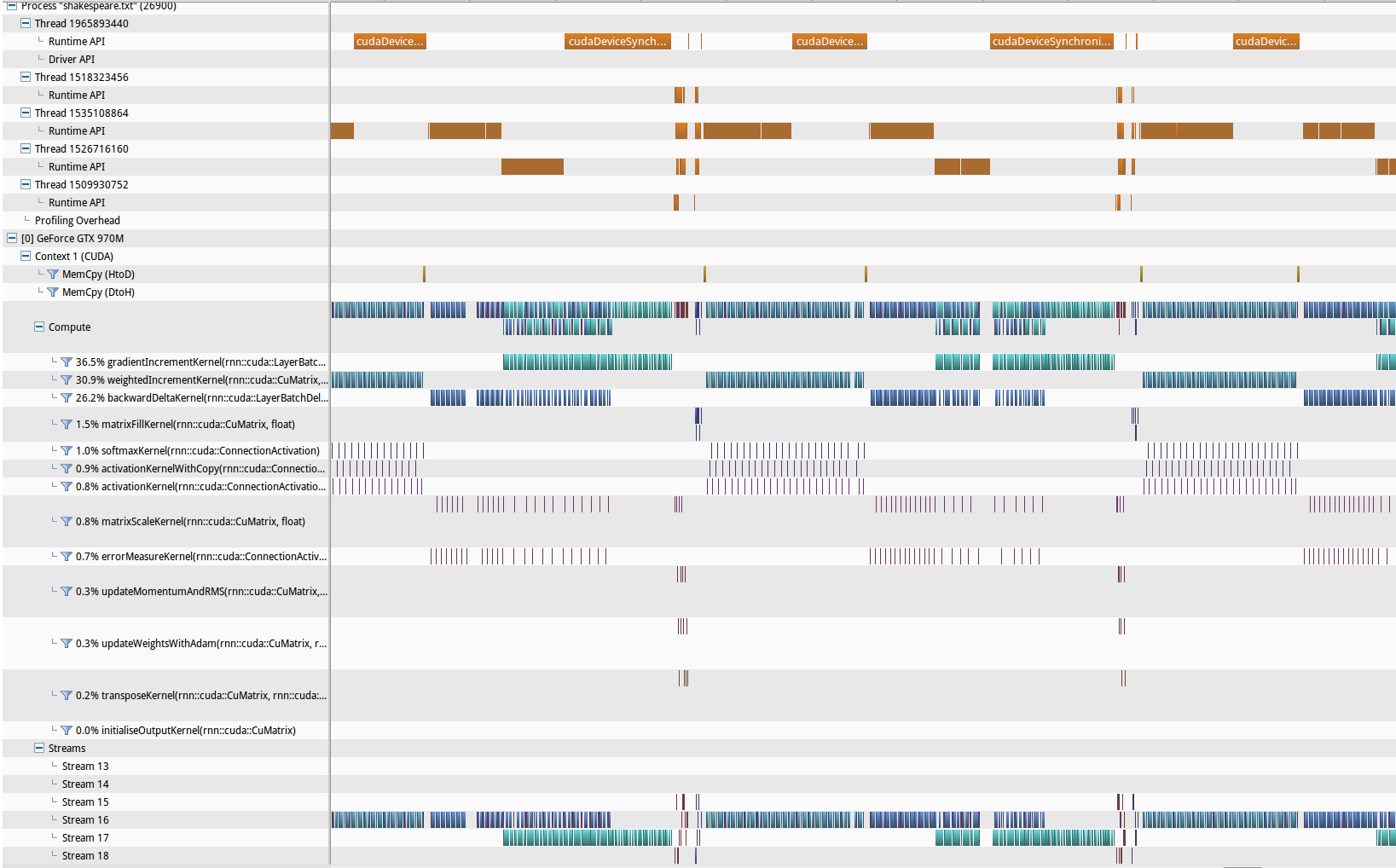
The first 3 are relatively straight forward and require little coordination and synchronization between streams. Splitting the forward (and back) propagation through the network across streams, however, is more difficult. The data dependencies here are based on the network structure, and doing this across streams is non-trivial. I decided to implement only the first 3 aspects, skipping the last one, in light of further performance investigation. The below NVProf analysis shows the improvements made in GPU compute utilisation.

Optimisation Caveats

So it was all well and good that I made some performance improvements by using some of the above techniques. However, at the end I realised/discovered it is mostly pointless. This is because the performance improvements largely disappear as the size of the network increases. This is because as the layers of the network become larger then the pure compute time to perform operations like matrix multiplication greatly overshadow any API call overhead or memory bandwidth under-utilisation. The performance improvements from the methods I used are apparent when the RNN has a couple of hidden layers of say size 32. But when the layers are size 512 then the pre-optimisations and post-optimisations versions are almost the same. In the case of these wider layers most of the time is spent in the kernels performing the operations, with the GPU at almost 100% utilisation throughout.

The code for this project can be found on Github: here and here (warning: code is experimental and may be slightly messy).