This is a very quick and dirty overview of Convolutional Neural Networks. I did not spend too much time working with these since currently my primary interest is focused on Recurrent Networks. But this quick writeup will serve for now for the sake of completeness…

Convolutional Neural Networks (CNNs) are a type of network that is especially well suited to problem domains with a spatially structured input, image classification being probably the most popular example. It is a problem-space that is quite well suited to the strength of neural networks, featuring a very high dimensional raw input that typically contains several “layers” of features (eg: edges -> corners -> faces). CNNs are feed-forward networks that are designed to take advantage of the inherent properties of this problem domain (CNNs are also used in other domains, but here I’ll focus mainly on image classification/recognition). The first property is that for object recognition there is (generally) translation invariance. That is, a cat in the top left corner of an image is still a cat if it was in the bottom right corner. Second we know that an object in an image has pixel locality. That is, a given object or “feature” (eg: edge or corner) tends to occupy a contiguous region of nearby pixels. Given these properties of the domain, a fully-connected network seems rather wasteful. (eg: it throws away all positional information about the pixels after the first layer). In this case there is a lot of background information that can be encoded into the structure of a Neural Network to improve its performance.

Weight Sharing and Convolutions

For Convolutional Nets, the main method of taking advantage of the domain structure is through weight sharing. Weight sharing constrains certain connection between nodes in a network to have the same weight value. CNNs use weight sharing in the form of “convolution layers”. A convolution layer is basically a set of independent feature detectors that are passed over the image pixels (or the output of a previous layer). A given “feature detector” of a convolutional layer will look at a small neighbourhood of pixels (say a 3x3 block). This neighbourhood of pixels is multiplied by a weights matrix, and then passed through an activation function. The “trick” comes from reusing the same matrix of weights for every 3x3 block of pixels, for a given “feature detector”. This is illustrated in the diagram below:

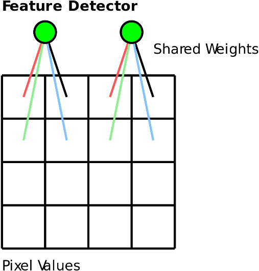
The above diagram illustrates a single “feature” detector that is a convolution over a 2x2 pixel neighbourhood. In this case, there are 4 weights associated with the feature. These same weights are used by the detector when processing different parts of the image. By doing this the feature detector can learn to detect a feature anywhere in the image, without having to “learn” translation invariance.

The convolution layers in a CNN function over a neighbourhood of the previous layers output, as well as over different channels of that output. A channel at the lowest level may be in the raw input, for example the individual RGB values of each pixel. A channel in a deeper layer would be the different features detectors from the previous layer.

It should be noted that the convolution neighbourhoods typically overlap, resulting in a convolutional layer’s output having the same (or similar) width as the input.

Pooling Layers

The Convolutional Layers of a CNN do not usually reduce the “width” of the data passing through the network, but instead add “depth”. The Pooling Layers are designed to reduce the “width” by performing some kind of summarization operation on a block of adjacent features. A simple example is a 2x2 max pool layer, where each node in the layer examines a 2x2 region of the previous layer and outputs the maximum value. An example of this is shown in the image below (taken from Wikipedia):

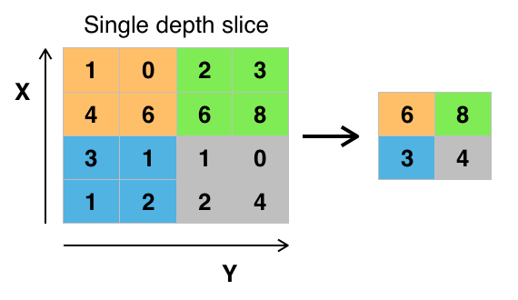
Typically these pool regions do not overlap (unlike the Convolution regions), so the effect of doing this is to reduce the spatial width of the data (if a 2x2 pool layer is used, the width of the network is halved).

Overall Network Architecture

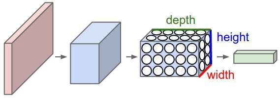
A CNN typically uses these two types of layers in tandem to build a larger network. The Convolutional and Pooling layers typically alternate, “squeezing” out the information from a wide stream of data (raw pixels) into a narrow but deep stream (diagram below taken from Andrej Karpathy’s webpage):

Depending on the specific image classification task being performed, the nodes in the deeper layers of a CNN will start to function as high-level object detectors. So for example you may have nodes that activate when the corresponding image region contains a face. After a number of layers of pooling/convolution, a CNN is typically suffixed with several fully-connected layers to perform the final classification task from the high-level features extracted by the convolution/pooling layers.

Applications

CNNs can be applied to a variety of problems, typically in the image/video recognition domain, but also in others where the incoming data has some spatial structure. One example is the AlphaGo program that beat Lee Sedol this year. In this case, I believe the neural network used to judge a particular board state was based on a CNN architecture. This makes sense, since in Go there are both low-level and high-level features with spatial locality, much like in image recognition (eg: Ko Fights).

I decided to have a quick play around with CNNs using the TensorFlow framework. This framework makes it quite easy to set up a straight-forward CNN with standard Convolutional and Pooling layers. I quickly hacked up a program for the standard MNIST digit recognition task. Even though this is a fairly boring and basically “solved” task, it is convenient in that I could compare the CNNs performance to my own fully-connected network implementations I’ve written previously (1) (2). In this case the CNN easily achieved an ~0.9% error rate on the test set, which is comparable to my fully connected network’s performance. The error rate can undoubtedly be reduced by further work.

I think for now I’m going to leave CNNs and focus more on agent control using RNNs. However, it’s possible to incorporate CNNs and RNNs together (for example to process a stream of images), so I may come back to this topic in the future.

The code for this project can be found on Github: here (warning: code is experimental and may be slightly messy).